In the last post, we made a T1-weighted image by driving the T2 term toward 1. To make a T2-weighted image, we do the mirror image of that trick: this time, we want the **T1** contribution to step out of the way and approach 1.

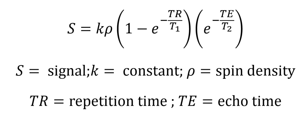
Look again at the T1 part of the equation, `(1 − e^(−TR/T1)). We want the entire term in parentheses to become 1. Remembering a bit of math, the way to get there is to make the exponential `e^(−TR/T1)` go to **zero**, because 1 − 0 = 1. And the way to drive an exponential toward zero is to make its exponent large and negative — in other words, use a **long TR**. In an equation:

With the T1 term forced to be close to 1, here is what is left standing in the original signal equation:

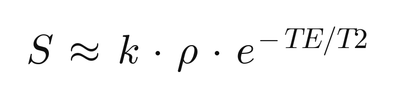
Now the signal depends only on spin density and on that last T2 term. To actually *see* T2 differences between tissues, we lean on `e^(−TE/T2)` by choosing a **long TE**. Tissues with a long T2 (fluid, edema) hold onto their signal and stay bright; tissues with a short T2 have already faded. That is the bright-fluid look you associate with T2. But, don’t get comfortable with T2 being associated with-bright fluid – more on that later. If you are reading this at your PACS station, pull up a “simple” T2-weighted sequence and check the parameters. You should see a **long TR** (typically a couple of thousand milliseconds) and a **long TE** (high double digits, often 80–100+ ms) — the exact opposite corner from the short-TR, short-TE T1 sequence.

So what happens if we keep the long TR but go back to a *short* TE? Let’s see that on the next post.