We have now used our equation to build two images by driving one weighting term to 1 at a time. What if we drive **both** of them out of the way at once? Do exactly that: keep the **long TR** from the T2 post (which sends the T1 term to 1), and borrow the **short TE** from the T1 post (which sends the T2 term to 1).

With both weighting terms sitting at 1, almost nothing is left:

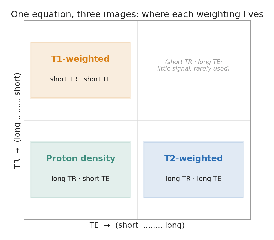
The signal now tracks `ρ` — the density of protons (mostly water and fat) in the voxel. This is the **proton-density** (or spin-density) image the first post promised was hiding inside every sequence. Because we have deliberately suppressed both T1 and T2 differences, PD images tend to show **less contrast** between soft tissues but carry a lot of signal, which is why they look smooth and a little “flat” while staying anatomically crisp. That trait makes them workhorses in musculoskeletal imaging (menisci, cartilage) and in the brain. In the brain, they have been mostly replaced by T2 FLAIR or fluid attenuated sequences.

If you are at your PACS station, pull up a PD sequence and confirm the pattern: a **long TR** paired with a **short TE**.

That completes the set. One equation, three images, sorted entirely by whether TR and TE are short or long:

We have been treating TR and TE as knobs without asking what they are physically doing to the signal. Next, let’s slow down and watch what TR is really doing.

Advanced note: If you pay attention to Radiology speak, you often hear of “PD/T2” combined as if they were one unit. It turns out, they are. The TE or echo time is the time at which a line of K-space is read out by the scanner. The actual readout time is pretty short, especially relative to the typically long repetition time or TR. So, if you were an industrious sequence, you could acquire BOTH a PD or T2 in the same TR. In fact, this approach is related to how we perform “turbo” sequences, such as the turbo spin echo.